Project

Install Libraries

pacman::p_load('tidyverse','tidyquant','tsibble','timetk','feasts','ggplot2','stats','lubridate','data.table','rmarkdown','knitr','nycflights13', 'dplyr')

Import Data Set

price_daily = read_csv("data/daily.csv")

paged_table(price_daily)

Time Series Analysis

This plot can be summarize by “week” or “month”

price_daily %>%
  dplyr::group_by(Country) %>%
  summarise_by_time(
    Date, .by = "week",
    Price = SUM(`Price (EUR/MWhe)`)
  ) %>%
  plot_time_series(Date, Price, .facet_ncol = 2, .interactive = FALSE, .y_intercept = 0)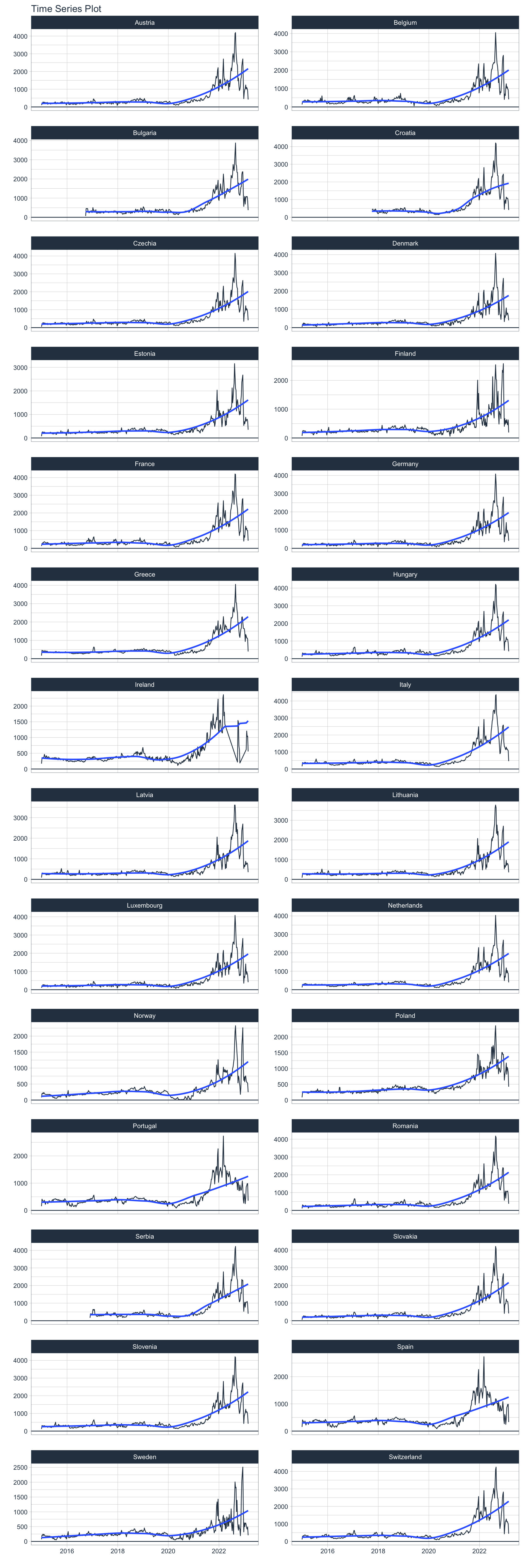

User is able to select countries and the time range

# Vector of country names to filter
countries_to_keep <- c("France", "Spain", "Italy")

price_daily %>%
  dplyr::filter(Country %in% countries_to_keep)%>%
  dplyr::group_by(Country) %>%
  filter_by_time(Date, "2021-06-01","2022-12-31") %>%
  summarise_by_time(
    Date, .by = "week",
    Price = SUM(`Price (EUR/MWhe)`)
  ) %>%
  plot_time_series(Date, Price, .facet_ncol = 2, .interactive = FALSE, .y_intercept = 0)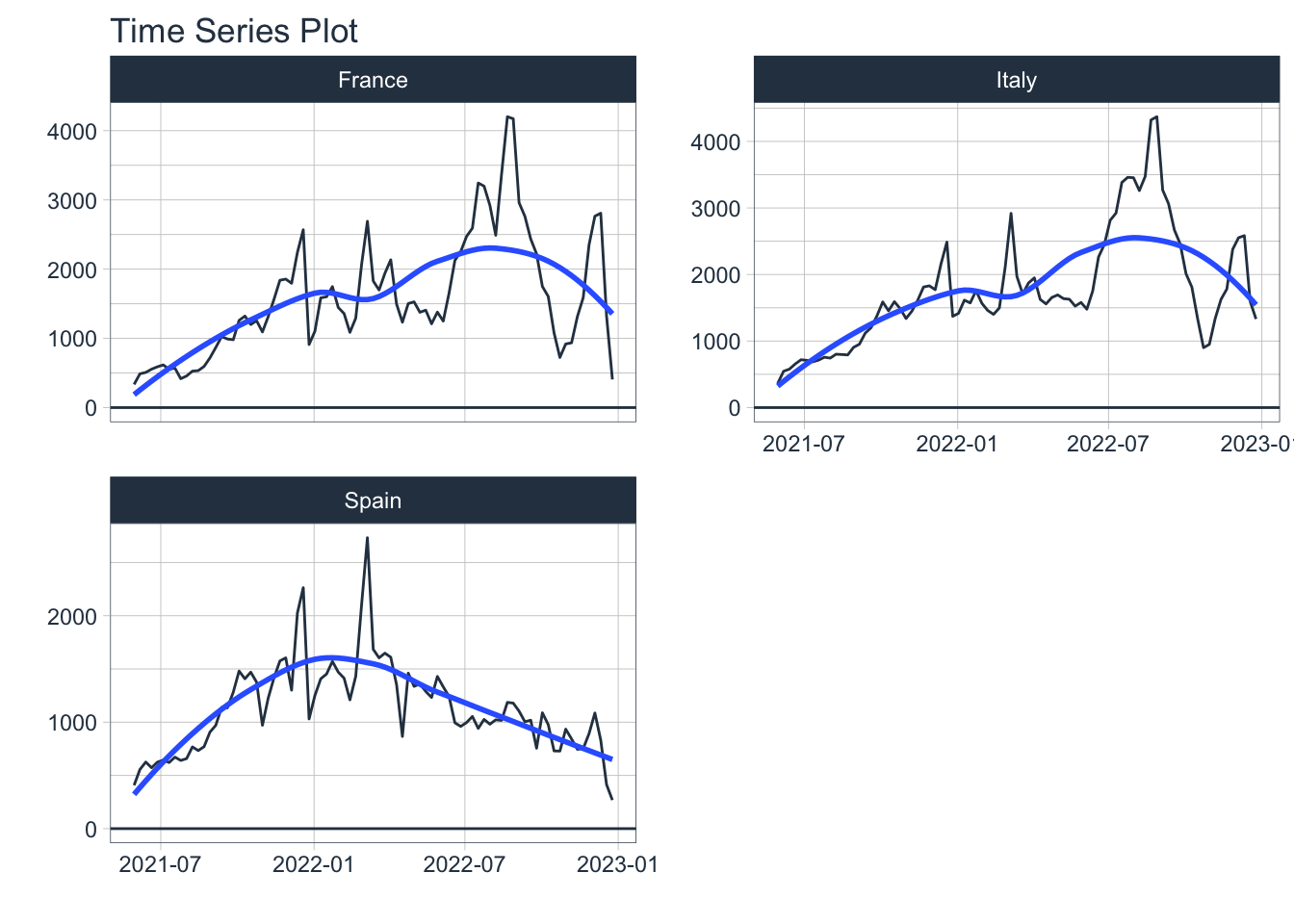

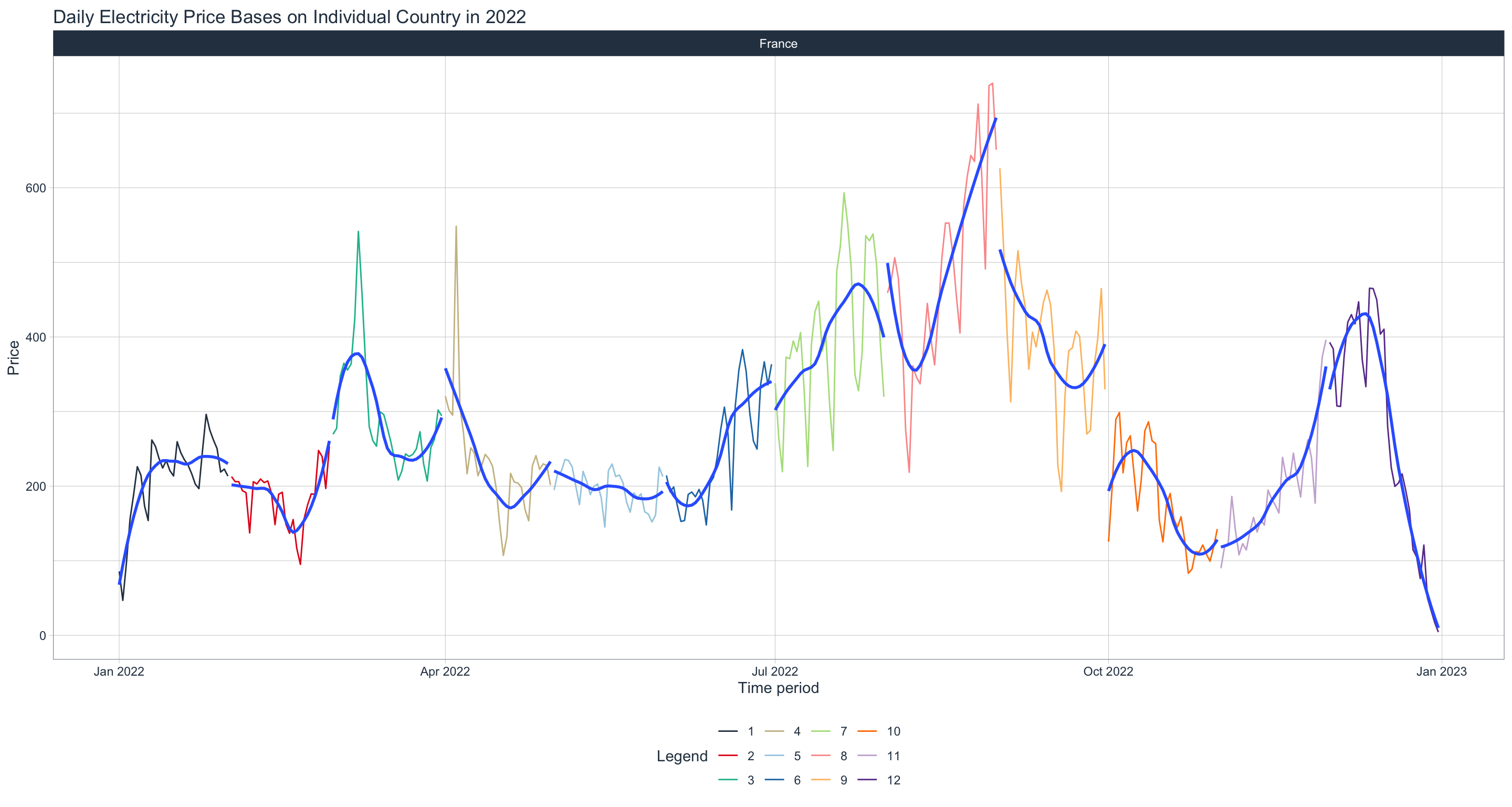
paged_table(price_daily)

Group Plot

User can edit Year and country

library(lubridate)

price_daily %>%
  dplyr::filter(Date >= as.Date("2022-01-01") & Date <= as.Date("2022-12-31")) %>%
  dplyr::mutate(month = month(Date)) %>%
  dplyr::group_by(Country) %>%
  dplyr::mutate(quarter= case_when(
      month >= 1 & month <= 3 ~ 'Q1'
      , month >= 4 & month <= 6 ~ 'Q2'
      , month >= 7 & month <= 9 ~ 'Q3'
      , month >= 10 & month <= 12 ~ 'Q4')) %>%
  dplyr::filter(Country=="France") %>%

  plot_time_series(.date_var=Date, .value = `Price (EUR/MWhe)`, 
                   .color_var = month (Date), 
                   .interactive=FALSE,
                   .facet_ncol = 2, .facet_scales = "free",
                   .title = "Daily Electricity Price Bases on Individual Country in 2022",
                   .x_lab = "Time period",
                   .y_lab = "Price",
                   .color_lab = "Month") + scale_y_continuous(labels = scales::comma_format()
                   )

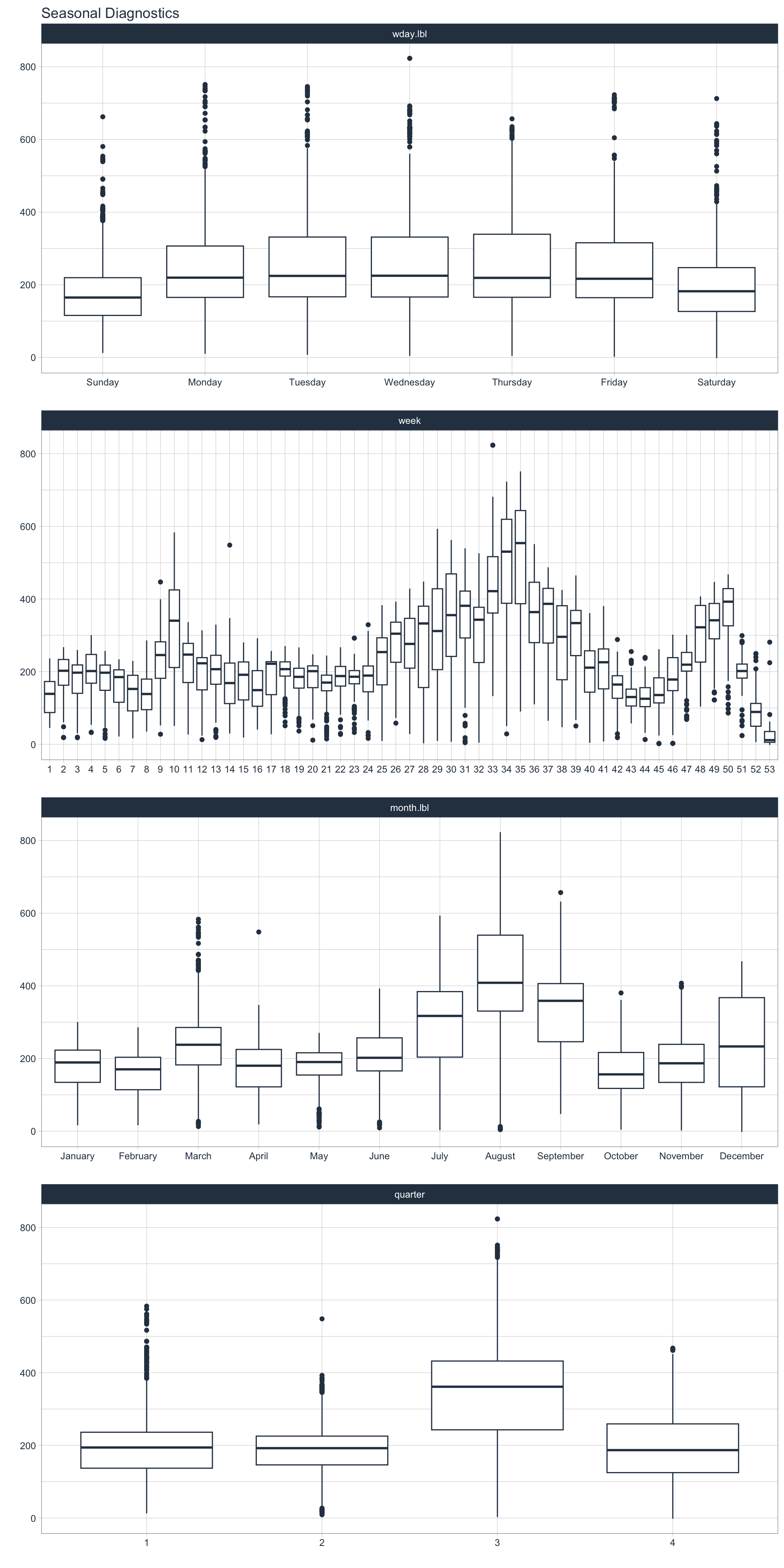
Seasonal Trends Analysis

price_daily %>%
    dplyr::filter(Date >= as.Date("2022-01-01") & Date <= as.Date("2022-12-31")) %>%
    plot_seasonal_diagnostics(Date, `Price (EUR/MWhe)`, .interactive = FALSE)