In-class Exercise 6

Author

Wang Ruipeng

Published

February 25, 2023

Modified

March 16, 2023

pacman::p_load(sf, tmap, tidyverse)

Import Data

mpsz <- st_read(dsn = "data/geospatial", 
                layer = "MP14_SUBZONE_WEB_PL")

Reading layer `MP14_SUBZONE_WEB_PL' from data source 
  `/Users/ruipengwang/Downloads/Chilly-RP/ISSS608-VAA/In-class_Ex/In-class_Ex06/data/geospatial' 
  using driver `ESRI Shapefile'
Simple feature collection with 323 features and 15 fields
Geometry type: MULTIPOLYGON
Dimension:     XY
Bounding box:  xmin: 2667.538 ymin: 15748.72 xmax: 56396.44 ymax: 50256.33
Projected CRS: SVY21

popdata <- read_csv("data/aspatial/respopagesextod2011to2020.csv")

popdata2020 <- popdata %>%
  filter(Time == 2020) %>%
  group_by(PA, SZ, AG) %>%
  summarise(`POP` = sum(`Pop`)) %>%
  ungroup()%>%
  pivot_wider(names_from=AG, 
              values_from=POP) %>%
  mutate(YOUNG = rowSums(.[3:6])
         +rowSums(.[12])) %>%
mutate(`ECONOMY ACTIVE` = rowSums(.[7:11])+
rowSums(.[13:15]))%>%
mutate(`AGED`=rowSums(.[16:21])) %>%
mutate(`TOTAL`=rowSums(.[3:21])) %>%  
mutate(`DEPENDENCY` = (`YOUNG` + `AGED`)
/`ECONOMY ACTIVE`) %>%
  select(`PA`, `SZ`, `YOUNG`, 
       `ECONOMY ACTIVE`, `AGED`, 
       `TOTAL`, `DEPENDENCY`)

popdata2020 <- popdata2020 %>%
  mutate_at(.vars = vars(PA, SZ), 
          .funs = funs(toupper)) %>%
  filter(`ECONOMY ACTIVE` > 0)

mpsz_pop2020 <- left_join(mpsz, popdata2020,
                          by = c("SUBZONE_N" = "SZ"))


write_rds(mpsz_pop2020, "data/rds/mpszpop2020.rds")

tmap_mode("plot")
qtm(mpsz_pop2020, 
    fill = "DEPENDENCY")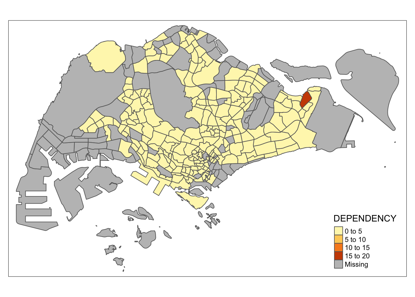

tm_shape(mpsz_pop2020)+
  tm_fill("DEPENDENCY", 
          style = "quantile", 
          palette = "Blues",
          title = "Dependency ratio") +
  tm_layout(main.title = "Distribution of Dependency Ratio by planning subzone",
            main.title.position = "center",
            main.title.size = 1.2,
            legend.height = 0.45, 
            legend.width = 0.35,
            frame = TRUE) +
  tm_borders(alpha = 0.5) +
  tm_compass(type="8star", size = 2) +
  tm_scale_bar() +
  tm_grid(alpha =0.2) +
  tm_credits("Source: Planning Sub-zone boundary from Urban Redevelopment Authorithy (URA)\n and Population data from Department of Statistics DOS", 
             position = c("left", "bottom"))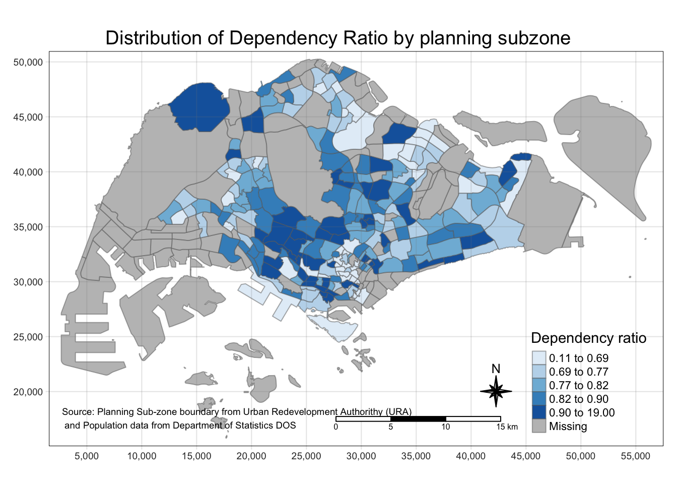

sgpools <- read_csv("data/aspatial/SGPools_svy21.csv")

sgpools_sf <- st_as_sf(sgpools, 
                       coords = c("XCOORD", "YCOORD"),
                       crs= 3414)

tmap_mode("view")
tm_shape(sgpools_sf)+
tm_bubbles(col = "red",
           size = 1,
           border.col = "black",
           border.lwd = 1)

tm_shape(sgpools_sf)+
tm_bubbles(col = "red",
           size = "Gp1Gp2 Winnings",
           border.col = "black",
           border.lwd = 1)

tm_shape(sgpools_sf)+
tm_bubbles(col = "OUTLET TYPE", 
          size = "Gp1Gp2 Winnings",
          border.col = "black",
          border.lwd = 1)

tm_shape(sgpools_sf) +
  tm_bubbles(col = "OUTLET TYPE", 
          size = "Gp1Gp2 Winnings",
          border.col = "black",
          border.lwd = 1) +
  tm_facets(by= "OUTLET TYPE",
            nrow = 1,
            sync = TRUE)